After much puzzling, I've made some progress on calculating the resistance between the diagonally opposite corners of a square laminar. Previously, I reduced this problem to solving
∇2u(x,y) = 0,
with boundary conditions
du/dn = 0, when x=±L or y=±L, and
u(-L,-L) = -1 and u(L,L) = 1.
This has the symmetry u(x,y)=u(y,x) and the antisymmetry u(x,y)=-u(-y,-x) which implies u(x,-x)=0.
Due to the antisymmetry, we need only consider the lower triangle with u(x,-x)=0 along the diagonal. Move this triangle so that the corner lies at the origin and duplicate it to fill all the quadrants.
We now have four lines of symmetry through the origin. These symmetries imply the Neumann boundary conditions on the internal triangle sides. This reduces the problem to solving ∇2u=0 over the whole diamond region with only the Dirichlet boundary conditions u=0 on the outer boundary and u(0,0)=-1.
Let's analyse the solution near the origin. If we're near the origin, we can regard L→∞. The problem becomes
∇2u=0 with u(0,0)=-1 and u(∞)=0.
This is conveniently radially symmetric so u=u(r). Using the polar form of the 2D Laplacian, we get
∇2u = u'' + u'/r = 0,
for r > 0. This can be solved by separation of variables. The solution is
u(r) = k ln(r) + c.
We must have k≠0 in order to have a nonzero current. The solution is therefore divergent at the origin which is incompatible with the boundary conditions.
There is no solution near the origin and therefore no global solution either.
Of course, a solution must exist in real life since I would surely be able to measure the resistance if I did the experiment. The problem is that I've modelled the situation incorrectly. In real life, the ohmmeter probes are not points but have a small size. We can assume the probes are conductive discs of radius s. This leads to a modified problem:
∇2u(x,y) = 0 on [-L,L]⨉[-L,L],
u(x,y) = 1 for (x-L)2 + (y-L)2 < s2,
u(x,y) = -1 for (x+L)2 + (y+L)2 < s2,
du/dn = 0 on the remaining boundaries.
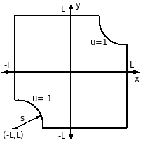
We again have the y=x symmetry and y=-x antisymmetry. We can rescale L=1 as long as we also rescale s → s/L = f.
We can transform the modified and rescaled problem as before:
If we assume f≪1, the solution near the origin is again
u(r) = k ln(r) + c.
Now the divergence at the origin is no longer a problem. The antisymmetry of the original problem implies c=0. To match the boundary condition u(f) = -1, we must choose
k = -1/ln(f).
The solution is then
u(r) = -ln(r)/ln(f).
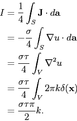
The current flowing into the probe can be found by integrating the current density. Using the four-fold symmetry of the transformed problem and a surface S surrounding the probe (shown in the diagram above), the current is given by
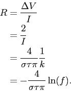
The resistance is then given by
Note that this result holds only for f≪1.
Without the rescaling, if we have a probe radius s, the measured resistance will go like
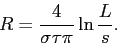
for L≫s. This contradicts [1] which states that the resistance is independent of L.
It appears difficult to find a general analytical solution for this problem due to the mixture of circle and triangle geometries. Instead, I have solved the equations numerically.
I implemented a finite difference method to solve the Laplace equation for u(x,y) on an NxN grid. I used second-order centered differences for the Neumann boundary conditions and the centered five-point differences for the Laplacian operator. This describes a sparse linear system which can be solved for u(x,y).
I used sparse matrix routines from UMFPACK to solve the system. I am impressed by UMFPACK's performance. It runs more than a hundred times faster than my own naive sparse solver. I used C++ bindings for UMFPACK from uBLAS.
The two symmetries can be exploited to twice halve the number of cells needed for the computation. (I've only implemented the antisymmetry so far though.)
Once u(x,y) is known, the current can be calculated using a surface integral over x=0. I used second-order finite differences to calculate J and used the rectangle method for the integration.
In order to get accurate results, the probe regions must occupy enough cells. Thus N must be chosen so that fN≳10. The program began swapping after N=1500 on my laptop with 2GB of RAM so I only have results down to f=0.005. I once tried running two N=3000 computations at the same time to exercise both cores of my Core 2 Duo T9300. This caused the laptop to overheat and switch off. An N=1500 computation takes about 1.5 minutes.
Here is a plot of the results:
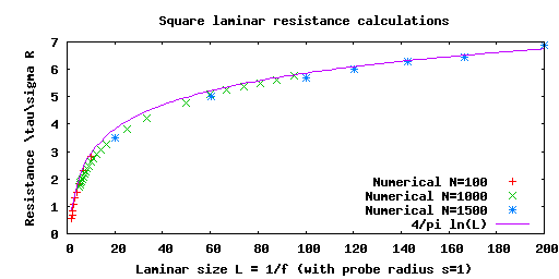
Our analytical calculation agrees with the numerical results for large L as expected.
We have two theories. [1] says R = 4/π 1/(τσ), independent of L. I say the resistance depends on L and goes like ln(L) for large L. Clearly the next step is to do an experiment to see who's right.
[1] Lawrence R. Mead, Resistance of a square lamina by the method of images, American Journal of Physics, 77 (3), (2009). Abstract